Introduction
What this guide is (and what it isn’t)
I wrote this guide when I joined a team where few people had formal training in forecasting methods, but many people had PhDs in quantitative fields and so weren’t afraid of a good-looking equation. As a result, this guide aims to help develop a solid mathematical basis on which to build data literacy and intuition for forecasting problems.
There are plenty of guides online for how to build forecasting model pipelines. Scikit-learn, a python library, made it possible to build a whole pipeline in 50 or so lines of code. However, the difficulty is in knowing: a) which 50 lines to write and b) what these 50 lines really do.
This guide aims to bridge the gap between what the python libraries tell you and what they don’t.
Here you won’t find: a cookbook with ready-made code examples available to plug and play with your data; strong opinions on which method is the best for all problems; or deep details on the underlying mathematics. However in here you will find: a wide survey of methods along with an overview of the mathematical underpinnings of forecasting, some historical context for the methods, and some free and paid resources to help further your learning.
The goal is to help you learn what is possible and what is available.
Note – Types of datasets: this guide sticks to dealing with tabular data (or data that can be transformed into a usual tabular format). This is in opposition to so-called unstructured data, like text or images.
What is forecasting?
The dictionary definition of forecasting is to predict or estimate a future event or trend. In our context, it’s specifically to make an educated guess about future data given our current data. This can mean predicting future prices with past prices, predicting future battery performance with past performance, or predicting future sales with past sales.
Note how this is different from building a physical model. Forecasting relies on capturing the information that exists in your data (sometimes you will also see people talk about capturing the signal in your data). Although physical modeling and forecast modeling are very different, they are both called modeling because they are both ways to represent the world.
Note – Physics-informed forecasts: Although I just spent a whole paragraph telling you that physics modeling and forecast modeling are different, there is a way to use both together. In fact, a physical model can inform the structure of your forecasting model. Steven Brunton has a nice youtube channel I recommend on this topic (and also a book which has been on my reading list for over a year, but who’s got time to read?)
It turns out there are many different problems we would like to forecast, and so there are many different forecasting methods. And adjacent to the forecasting methods, there are approaches to test for the validity of the forecasting methods. A full forecasting model is usually, a method (like linear regression), a testing framework (like cross-validation), along with some data (and associated feature engineering).
Fundamentally, forecasting methods rely on the assumption that there is a stochastic element to data collection. Out of all the possible asset prices, we saw only the ones that did happen. The question becomes, how different could the prices have been? And in the future, how different can they be? And how do past prices relate to future prices? Forecasting is about exploiting the inherent stochasticity in our data to answer these questions.
Note – Frequentists VS Bayesians: The above paragraph is mostly written from a frequentist perspective, which is the dominant framework people learn. This reformulation relies on the idea of repeated sampling while a bayesian version of this would rely on the idea of measuring uncertainty (i.e. what is our belief about what the prices could have been).
What does solving a typical forecasting problem look like?
First, you would perform Exploratory Data Analysis (EDA). Often, this means plotting your data and looking at simple metrics: min, max, mean, standard deviation, quantiles, correlation across variables, … This allows you to start to guess at some of the rules that your data follows. Then, using domain expertise you would start to narrow down which kind of problem we are facing. What do we want out of our data? How much data do we have? How explainable do we need our solution to be? What’s the measure of success for our forecasting model? The answers can change over time, and this is reflected in our choice of modeling approach.
Generally, before building a complex model and once the questions we want to answer are clearer, we start by building a simple benchmark. This benchmark should be as simple as: using a mean; using the previous day’s data; using a fixed prediction; a very bare bones linear regression. Without such a benchmark, we don’t even know what we are aiming to beat.
Once we have a benchmark and we have some idea for a more complex model, there are generally three avenues to augment that more complex model:
-
Feature engineering:
That is, modify your data in some ways. This is usually driven by the results of your EDA and your domain expertise. For instance, if you know that markets behave in a certain way, you can modify your market data to reflect that. Modifications can be about removing outliers, scaling the data, generating interaction variables, or passing your data through a complex function. A variety of metrics from the world of information theory can help you assess if your transformed data is better for the forecasting task. Note that usually the number of possible transformations is much higher than what any computer can handle, so you need to exercise judgment when coming up with them.
-
Tune your model’s parameters:
We will cover more examples of model parameters later, but this tuning is an essential step. Although it depends strongly on your data, it is also very much about the specific model you are using.
-
Finally, try a different model:
There are different models to try for regression or classification, and their quirks will fit some problems better than others. A priori it is usually hard to guess which model will perform best.
Note – What constitutes a model: is it the base equation? Is it just the parameters? Is it the trained output of your code? Is it how you train and test the model? Is it your data? Most people nowadays agree that it is all of that, and so you should have a versioning system to make sure you know at all times which version of your data goes with which version of your model training approach.
Note – Feature engineering: Machine Learning will often perform drastic data transformations to build models with better out-of-sample performance. This data transformation is often called feature engineering, or feature extraction, or sometimes more specifically dimensionality reduction. Feature engineering can mean taking a continuous variable (e.g. age number) and making it into a categorical variable (e.g. age category like child, adult, …) via heuristics, or it can mean using statistical methods to create the features. Econometrics however tends to be much more restrained with its data transformations, typically takings logs or first-differences only.
Notations
The most striking thing I learned about mathematics in high school is that notations are everything. It’s happened to me before to pick up a textbook or start a maths class and to not understand about the notation and have to google everything. Hopefully this section avoids you these pains.
Matrix notation
Scalars are like regular numbers, while vectors are collections of scalars. We say vectors are of shape \( n \times 1 \) where \( n \) is the number of scalars in the vector. Matrices are collections of vectors. We say a matrix has shape \( n \times k \) when it has \( n \) rows and \( k \) columns.
Typically, scalars are designated by a single lowercase letter, while vectors are a single lowercase letter with either an arrow above or in bold, and matrices are a single uppercase letter, sometimes in bold. When the context makes it obvious, the arrow or the bold font are omitted for legibility. Confusingly, random variables are also denoted by a single upper case letter. Welcome to statistics.
If you want to use words, tensors are the 3+ dimensional equivalent of matrices.
Transpose notation
The transpose of a vector or of a matrix is that same vector or matrix but flipped symmetrically along its diagonal. So a vector that is \( n \times 1 \) becomes \( 1 \times n \) and a matrix that is \( n \times k \) becomes \(k \times n \). The notation for the transpose of matrix \( X\) is \( X’ \) or sometimes \( X^T \). In this guide I use \( X’ \) for legibility.
Distribution notation
To indicate that a random variable \( X \) follows a given distribution \( \mathbb{F} \), the notation is: \( X \sim \mathbb{F} \).
Matrix operations VS scalar operations
Multiplying two numbers together is easy, but to multiply two matrices or vectors, their sizes need to match up: if \( X\) is \( n \times k \) and \( \beta \) is \( k \times 1 \) then I can compute \( X \times \beta \) and the result is of size \( n \times 1 \), but I can’t compute \( \beta \times X \). Note how squaring matrices works: \( X^2 \) can be either \( X’X \) or \( XX’ \). You choose the one you want based on the dimensions you want and/or need for your result. Note that this means that squaring a vector can lead to a scalar or a square matrix.
Hat, tilde, dot
In a forecast, we typically estimate parameters. If the true parameter is written as \( \beta \) then the estimated parameter will be written with a hat: \( \hat{\beta} \). Some data transformations are written using a tilde above the variable that represents the data. Data transformations that involve differencing typically use dots instead of tildes, which is a convention that comes from the field of differential equations.
- Hat: \( \hat{\beta} \)
- Tilde: \( \tilde{x} = f(x) \) where f is some function
- Dot: \(\dot{x}_{t} = x_{t} – x_{t-1}\)
Derivatives
Usually, a derivativate is denoted using \( ‘ \), but to not create confusion with the transpose notation and to be more explicit on the number of times the derivative is taken, I use the notation \( X^{(n)} \) to indicate the \( n-th \) derivative.
Population or sample data
Throughout the guide, I talk about population data and sample data. The population is the entire data that can, while the sample data is the part of that total that I collected.
For instance, if I measure the height of everyone in a building, that is a sample of all the heights that are possible for people. Note that the definition of population data can be difficult: it could be all the people currently alive, or all the people ever. How far back do we go? Up until homo sapiens first appears? Such considerations are usually important insofar as it’s important to understand if the data that was collected was collected because it was special in some way (e.g. is there some selection bias at play).
Consider a maybe less contrived example. In the stock market, we observe only one price for each time of the day for each asset. What is the population distribution for that data? Is it a distribution for each time? What if some times have no new prices? Is it a distribution for each day? Is it a distribution for each asset? It’s unlikely that there is a true answer here, rather what matters is what we’re trying to model.
Expectation, variance, covariance
The operator \( \mathbb{E} \) is called the expectation, or expected value, and it is (usually) equivalent to the mean. The variance operator is most often written \( Var \), and the covariance operator \( Cov \).
Conditional notation
Sometimes, we want to express what we know about a random variable given some knowledge we already have, as opposed to without that knowledge. Consider the random variable \( Y \), and some information \( X \). We write formally that \( Y \) given \( X \) is \( Y | X \).
Machine Learning and Econometrics
Why bother with Econometrics
Nowadays, almost all the best forecasting methods come from the field of Machine Learning (ML). So why bother with an old field like Econometrics? Although it’s often true that Econometrics methods perform less well (specifically when measuring out-of-sample performance), they are often much more explainable. Moreover, the mathematics of ML tend to focus on numerical computation while the mathematics of Econometrics tend to focus on analytical solutions to modelling problems. As a result, the two tool sets complement each other well.
Econometrics
Historically, Econometrics came first. It can be considered a sub-branch of Statistics and Economics. Some classic questions for Econometrics are:
- Given some past price data, can I predict future price data?
- Given an equation for how unemployment and inflation are linked, can I estimate the parameters of this equation?
- Can I evaluate the existence/validity of the causal link between seemingly unrelated data?
Because Econometrics is older, it concerns itself a lot with:
- Causality and how to recover it from data, in the context of explaining in-sample effects.
- Estimation with small datasets (Economics departments used to have armies of grad students invert matrices by hand).
- Analytical solutions and other theoretical results (e.g. BLUE estimators).
Machine Learning
Machine Learning is a more recent field and is usually considered a sub-branch of Statistics and Computer Science. Machine Learning concerns itself more with issues of pattern recognition. Some classic questions for Machine Learning are:
- Given different classes for my data, can I predict the class of a new piece of data?
- How well does my prediction generalize outside of my training data?
- Can I use the features of my data to come up with a classification?
Because Machine Learning is more recent and is more in line with modern computing advances, it concerns itself a lot with:
- Numerical solutions to problems (e.g. gradient descent).
- Out-of-sample predictions and predictions on very different data (i.e. overfitting).
- Applied heuristics (e.g. how to select a best model in practice, regardless of theory?).
Nowadays both fields can and should use each others’ tools. In practice, both can tend to look down on each other. ML practitioners think Econometricians don’t know how to use computers properly and Econometricians think it’s crazy that people don’t seem to care about causality or statistics anymore.
Supervised or unsupervised learning
Some examples of problems and their solutions
-
Can you predict future energy prices with past prices and weather forecasts? Linear regression approach:
- Strong model assumption of linearity
- Distributional assumptions built-in, so immediate hypothesis tests and confidence intervals
- Easily explainable
Random Forest approach:
- Less overfitting, no parametric formula assumptions
- Less explainable (SHAP can explain feature importance but is flawed)
- No confidence intervals unless we bootstrap, requiring more data and/or compute
-
Can you predict whether a bus’s battery will last until the end of a trip?
Polynomial or Exponential regression to fit battery discharge behavior on given road:
- Strong model assumptions closely fit our physical understanding
- Granularity of prediction during the ride
- Easily explainable
Classification approach:
- Easy to compute even before the trip based on battery, vehicle, and route indicators
- Very easy to communicate
- Simple 0 or 1 indicator, but not very granular
Regression
Why focus on regression analysis
In the next section we will spend a significant amount of time on regression analysis and its mathematical underpinnings. The reason for this choice is four-fold:
- Regression is a somewhat simple model with strong mathematical underpinnings. These assumptions are very useful for understanding what we want in a “well-behaved” model, not just for linear regression.
- Regression has a lot of extensions. It can be linear or have many different shapes, it has extensions that allow for parameter shrinkage and automatic selection (see elastic net later on), and overall offers a surprisingly flexible and explainable framework. Even in cases where the ultimate model is not linear regression, I still find myself thinking about a lot of the concepts I explain here when making sure my random forest or support vector machine is working correctly.
- A lot of classification models can be represented with a regression set up (e.g. logit or probit).
- That’s how I learned forecasting, so I’m biased.
Note – What does the word regression mean?: You may have heard the term regression towards the mean, and you might know that regression in most contexts means going back or reverting. Regression towards the mean is when you sample data from some process, let’s say you measure people’s heights, and you observe a really large number, say someone measures above 2 meters. Then you would expect your next sample to not be so extreme, and instead be \closer\ to the mean value, in our example the mean height.
History
Regression was officially discovered and published by Adrien-Marie Legendre in 1805, although Gauss is rumored to have used the method in his work up to 10 years before and is credited with significant advancements to the method. The method originally came from the fields of astronomy and geodesy, and in particular came about to solve the challenges of navigating the Earth’s oceans during the Age of Discovery.
The problem to solve was the following: given some features \( X \), a \( n \times k \) matrix, and some outputs \( y \), a \( n \times 1 \) vector, can you find the link between \( X \) and \( y \)? Nowadays Econometrics also really cares about whether that link is causal (which is arguable not a mathematics question), but the fundamental mathematical problem is to estimate that relationship.
The problem they set out to solve is to find \( \beta \) such that:
\[y = X \beta + \varepsilon \]
This equation is often called the regression anatomy formula.
Another way of looking at it, is to think about defining the shape of the error that you are willing to live with:
\[\varepsilon = y – X \beta\]
Note that \( \varepsilon \) is \( n \times 1 \) and \( \beta \) is \( k \times 1 \).
Furthermore keep in mind that the fundamental goal of linear regression is to reduce the dimensionality of your problem. Reducing a scatter of points to a single line loses some information. The data is not allowed to move in some directions as a trade-off to make the problem more explainable. Ideally all the movement removed is represented by the error term, but that is not always true.
Note – Linear VS non-linear regression: What makes the regression linear? Above, we saw that we can interpret regression as defining the shape of error we can live with. If that function is linear in \( X \), then the regression is said to be linear. In practice, this is visible because if you draw your regression line, it will be straight. This consideration is separate from how we measure our error term (vertical, perpendicular, squares, etc), as discussed in the next section.
How would you solve this?
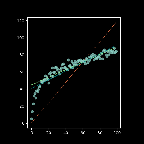
Looking at the image below with a linear scatter: where would you put the line of best fit?
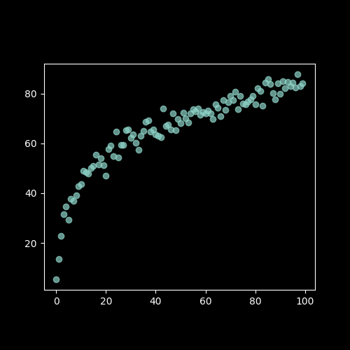
If we draw a straight line through these points, then the distance between the points and the line is our error. Ideally we would want the total error, i.e. the sum of those distances, to be minimized. This idea of minimising a sum of error terms is key to most ML methods.
Visually, that error can be represented by line segments that start at our data points and go towards the fitted line. But which orientation should the segments have?
The segments could intersect with the line of best fit perpendicularly:
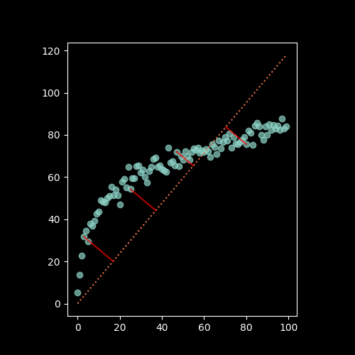
Or the segments could all be parallel to one of the axes:
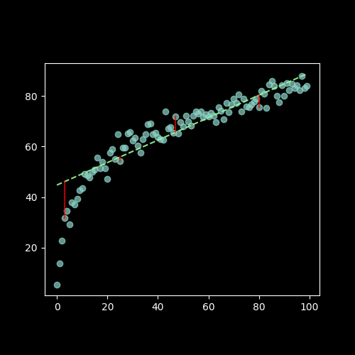
Gauss and Legendre’s insight was to draw not line segments, but squares, and to find the line that minimizes those squares:
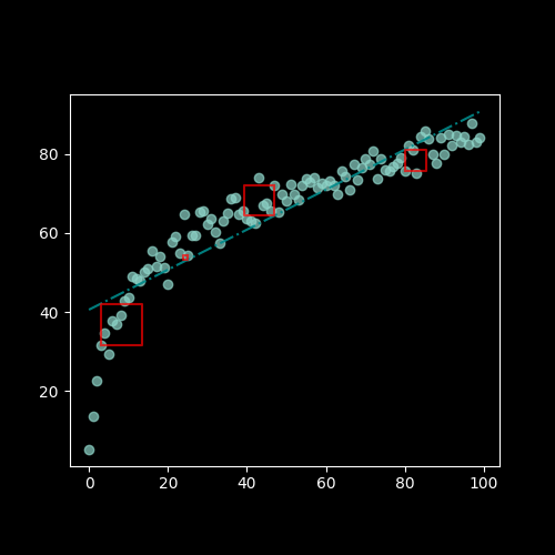
Look at how different those lines look like:
Fundamentally, there are two considerations:
- Which direction the error lines are pointing – we saw vertical and perpendicular, but horizontal is also possible. A vertical line (i.e. parallel to the y-axis) implies that we only consider errors for the \( X \) variables, while a horizontal line (i.e. parallel to the x-axis) implies that we only consider errors for \( y \) variable. A perpendicular line implies that we consider the errors for both the \( X \) and \( y \) variables. Whether the line segment is vertical, horizontal, or perpendicular changes the regression anatomy formula.
- How we sum our errors – the most common ways are the Mean Squared Errors (MSE) and the Mean Absolute Errors (MAE). For the MSE, we square our errors and then sum them, while for the MAE we take the absolute value of our errors and then sum them. More formally:
\[MSE = \frac{1}{n} \sum_{i=1}^{n} \left( \varepsilon_i \right)^2 = \frac{1}{n} \sum_{i=1}^{n} \left( y_i – x_i \beta \right)^2 \] \[MAE = \frac{1}{n} \sum_{i=1}^{n} | \varepsilon_i | = \frac{1}{n} \sum_{i=1}^{n} | y_i – x_i \beta | \]
Where \( y_i \) is a scalar and \( x_i \) is a vector, making the MSE and MAE scalars.
Using vertical lines and squaring them to minimise the MSE is how we obtain the most commonly known regression formula: Ordinary Least Squares (OLS). But of course, all other set-ups are allowed: horizontal errors with the MAE, perpendicular errors with the MSE, etc. That last one is called total regression, or sometimes orthogonal regression or even Deming regression. It is rare to see it in practice as a form of regression, and instead this approach is more commonly seen in ML methods such Principal Component Analysis (PCA) or Support Vector Machines (SVM).
For now, we focus our attention on OLS, and why the insight of minimising squares is so powerful:
- Squaring your errors before adding them together means that positive errors and negative errors do not cancel each other out.
- The square function is easy to differentiate, so we can look at our estimated errors, square them, and taking the derivative, we can easily derive our estimator for \( \beta \) analytically. Compare this with the MAE, which has a kink around 0 and is therefore not easily differentiable.
- Squaring is how we calculate the Euclidian distance in an arbitrary vector space. Looking at the vector space spanned by \( X \), squaring the elements is like computing the \( L2 \) norm. In particular, you can prove that minimizing the \( L2 \) norm is a type of projection onto a vector space. And since minimizing the \( L2 \) norm is how we solve for our OLS estimator, we can understand OLS as a projection of \( y \) onto the vector space spanned by \( X \). This gives us a strong geometric representation of what our approach does.
Key Theorems
We now turn our attention to the two key results needed for classical linear regression to work nicely: the Law of Large Numbers (LLN) and the Central Limit Theorem (CLT). Both are limit theorems but the former is about point estimation while the latter is about distributional estimation.
LLN
\[ \lim_{n \to \inf} \frac{1}{n} \sum_{i=1}^{n} x_i = \overline{X}_n = \mathbb{E}[X]\]
The main intuition behind the LLN is that if you repeat an experiment enough times, the average value of the samples is the true average. More specifically, this theorem makes use of mathematical limits and claims that as we get more data, we converge to the true average.
CLT
\[ \lim_{n \to \inf} \frac{\sqrt{n}}{\sigma} \left( \overline{X}_n – \mu \right) \sim \mathcal{N}(0,1) \]
The main intuition behind the CLT is that if you repeat an experiment enough times, you know how the average of those experiments will behave. More specifically, the distribution of the average value of the samples follows a normal distribution.
Historically, the normal distribution and the mean are two very well-understood tools in statistics. As a result, the LLN and CLT work together as the building blocks of many forecasting methods. They are the reason why having more data is better. It’s better in fact because these are limit theorems, and more data (should) mean better convergence. In practice, finite sample properties of limit theorems are not always very well-behaved. There are heuristics to deal with this, but in general:
- For Econometrics methods using OLS, 300 data points can be enough
- For ML methods using trees, 1 000 data points can be enough
These two theorems together guarantee a wide variety of desirable properties for linear regression (i.e. BLUE estimator via the Gauss-Markov theorem). However, these two theorems are also what allows bootstrapping and neural networks to work. They really underpin the whole field of estimation. Here I’ve expressed these ideas using the Frequentist framework, but these theorems also Bayesian equivalents.
The next section covers assumptions needed for our OLS estimator to be well-behaved. These assumptions are chosen in large part for how they rely on the LLN and CLT.
Note – Why is there no \( n \) on the right hand side of the limit equation? For many years, I was told it’s bad form to have the \( n \) there, with no better explanation. It’s not until reading The Simple and Infinite Joy of Mathematical Statistics that I saw a good reason: once you take the limit in a given variable, it is gone from your expression! For years that convention was nagging at me just enough to stay in mind, not enough to actively seek out the reason, but now I (and you) know.
The OLS estimator
There are many equivalent ways to derive the Ordinary Least Squares estimator for a linear equation. Here we take the square of our errors and differentiate them. Setting the derivative equal to 0 allows us to solve for the \(\beta\) that minimizes the errors. We check that this is indeed the minimum by taking the second derivative. Note that the following is written in matrix notation, so \(\varepsilon’ \varepsilon\) is really \(\varepsilon^2\). Note how \(\varepsilon’ \varepsilon\) is a scalar. We start with the first order condition:
\[\mathop{\arg\min}\limits_\beta \hspace{2mm} \varepsilon’ \varepsilon = \mathop{\arg\min}\limits_\beta (y – X \beta)'(y – X \beta) \quad (1)\] \[\Leftrightarrow \frac{d}{d\hat{\beta}} \left[(y – X \hat{\beta})’ (y – X \hat{\beta}) \right] = 0 \quad (2)\] \[\Leftrightarrow \frac{d}{d\hat{\beta}} \left[y’y – y’ X \hat{\beta} – \hat{\beta}’ X’ y + \hat{\beta}’ X’ X \hat{\beta} \right] = 0 \quad (3)\] \[\Leftrightarrow \frac{d}{d\hat{\beta}} \left[y’y – 2 \hat{\beta}’ X’ y + \hat{\beta}’ X’ X \hat{\beta} \right] = 0 \quad (4)\] \[\Leftrightarrow – 2 X’ y + 2 X’ X \hat{\beta} = 0 \quad (5)\] \[\Leftrightarrow X’ X \hat{\beta} = X’y \quad (6)\] \[\Leftrightarrow \hat{\beta} = (X’X)^{-1}X’y \quad (7)\]
From (1) to (2), take the first derivative to find the \( \arg\min \). Use \( \hat{\beta} \) to indicate the estimator as opposed to the true value. Note that this whole expression is a scalar, it is equal to the number 0, not a matrix of 0s. This means we can take transposes of each element.
From (2) to (3), expand the terms.
From (3) to (4), rearrange the scalar terms to group them by exponent of \( \beta \).
From (4) to (5), apply the derivative.
From (5) to (6), move over the terms by adding on both sides and dividing by 2 on both sides.
Finally from (6) to (7), multiply by the inverse on both sides.
Now we look at the second order condition: \[\frac{d^2}{d\hat{\beta}^2} \left[(y – X \hat{\beta})’ (y – X \hat{\beta}) \right] = X’X > 0\]
So the estimator does in fact minimize the squared error.
The complete derivation is only included to satisfy the more curious readers. For those who want some extra credit, look into two other ways of deriving this same estimator: the method of moments and the maximum likelihood estimation method. Regardless, the most important thing to remember from this derivation is the final formula: \[\hat{\beta} = (X’X)^{-1}X’y\] Most crucially, note the need for matrix inversion. A lot of estimation methods rely under the hood on matrix inversions, which is one of the reasons why inverting matrices is such an important aspect of modern computing.
In the next section, we look in detail at the assumptions that make OLS the best estimator.
Assumptions deep-dive
A few assumptions are required so we can use our theorems to make OLS a valid estimation method. These assumptions are sometimes labeled A1 to A5 (A for assumption) and have a few variations. I list all these assumptions in quite a lot of (mathematical) detail here in an attempt to provide a mathematically solid intuition.
- A1: \( X \) is a \( n \times k \) matrix with rank \( \rho(X) = k \), i.e. it has full rank
The rank of the matrix refers to how many true columns there are in the matrix. Remember that the columns in \( X \) are the features, so this is really a statement about the validity of our features. A classic case where this rank assumption is violated is if one column can be written as a linear combination of other columns, then that column contains redundant information and it wouldn’t count towards the rank of \( X \).
Consider the case where one column is \( age \), and another column is \( age \times 2 \). The second column does not contain any new information. Another example would be a column for \( salary \), a column for \( years\_of\_study \), and a third column which is \( salary + years\_of\_study \times 10 000 \). That third column contains fundamentally the same information as the first two. This issue is also particularly common when creating categorical variables and including all the categories. Note however how this only applies to linear combinations. A column like \( age^2 \), or \( salary \times years\_of\_study \) would not be a linear combination of other columns because two columns are multiplied together. These are actually valid and often useful transformations. - A2: The model is linear and can be written as\( y = X \beta + \varepsilon\) with \( \mathbb{E}[\varepsilon] = 0 \)
This assumption is about the shape of the model. We assume a linear relation between our features and our outcomes. Note that the condition on the expectation of \( \varepsilon \) is easily obtained by taking advantage of the fact the \( \mathbb{E} \) operator is linear. Consider the case where \( \mathbb{E}[\varepsilon] = \mu \), you can rearrange your terms to redefine \( \tilde{X} = X + \mu \), and \( \tilde{\varepsilon} = \varepsilon – \mu \) and satisfy that condition.
- A3: The different features (i.e. columns) in \( X \) are “unrelated” or “exogenous” with respect to \( \varepsilon \)
This assumption is about making sure that the errors do not actually contain signal. A classic case where this happens is when there is another feature that is not included in \( X \) but is correlated with the features in \( X \). Consider running a regression of \( salary \) on \( years\_of\_schooling \). \( age \) is most likely correlated with both \( salary \) and \( years\_of\_schooling \) but is not included in the features. This means that \( \varepsilon \) will be correlated with our \( X \). We call such variables confounders, and when forgotten they introduce bias in our estimate for \( \beta \).
A3 comes in different flavors. Here they are, in order where the first one is the strongest assumption and the last one is the weakest (in the sense that the stronger assumption implies the weaker one). The details of what this means for the estimator \( \beta \) is out of the scope of this guide, but I think it can be useful to see how subtle differences can actually mean a lot:- A3F: \( X \) is non-stochastic or fixed in repeated samples.
This is when \( X \) is actually not a random variable. For the cases we concern ourselves with, this is almost never the case. However it shows how all of our estimation techniques rely on our data being stochastic.
- A3Rfi: \( X = {x_{i,j}}, \forall i, j \) are random and mutually statistically fully independent from \( \varepsilon_i \).
Note how this independence is across features and across individuals (i.e. across the columns and across the rows). This is a very strong assumption and is almost never true, simply by virtue of the fact that most things are correlated in life.
- A3Rmi: \( X \) are random and with \( \varepsilon \) are vector mean independent, i.e. \( \mathbb{E}[\varepsilon | X] = constant \) (that constant must be 0 from A2).
Note first that I use vector notation here, meaning that the independence holds across individuals (i.e. across rows). Secondly take note of what the conditional expected value means: I can’t learn more information about \( \varepsilon \) by adding that I know X.
- A3Rsru: \( X = {x_{i,j}} \) are random and with \( \varepsilon \) are same row uncorrelated, i.e. \( \mathbb{E}[\varepsilon_i x_{i,j}] = 0 \forall i,j \).
Note that this is no longer vector notation, so there could be some correlation across the rows between our features and our errors. These are sometimes referred to as spillover effects and they are the bane of randomized control trials. Note also that we don’t write this as a conditional expectation, but as a multiplication. In practice, \( \mathbb{E}[\varepsilon_i | x_{i,j}] = 0 \forall i,j \) would be a different stronger assumption, but in practice we would use it to show that the product is 0. This is the part that matters mechanically for getting rid of bias terms.
- A3F: \( X \) is non-stochastic or fixed in repeated samples.
- A4: The variance of the errors is of a known shape
We now look at assumptions on the covariance of the errors. Just like A3, the following are in order of the strongest to the weakest assumption:
- A4GMiid: \( \varepsilon_i | X \) are identically and independently drawn and all moments of \( \varepsilon \) are finite.
Moments are key statistics of distributions and generalize the idea of mean and variance. The mean is the first moment, the variance is the second moment, the skewness is the third moment, and the kurtosis (i.e. the tailedness) is the fourth moment. The number of the moment refers to the largest polynomial used to compute it. The mean uses a power of 1, while the variance a power of 2, etc. This assumption implies that all individual \( \varepsilon \) have the same mean, variance, etc. The moments being finite is very important as that condition is needed for the LLN and CLT to work properly. In practice, we never get infinite values, but we can still get numerically unstable ones.
- A4GM: \( \mathbb{E}[\varepsilon \varepsilon’ | X] = \sigma^2 I_n \) where \( \sigma < \inf \) (i.e. the second moment is finite).
Here \( I_n \) is the identity matrix of size \( n \times n \), so really this means that we have the following properties for our errors: (i) homoskedasticity: \( \mathbb{E}[\varepsilon_i^2] = \sigma^2 \)n, so our errors have the same variance regardless of our \( X \) and (ii) no autocorrelation: \( \mathbb{E}[\varepsilon_i \varepsilon_k] = 0 \forall i \ne k \), so our errors are not correlated across rows with each other.
- A4 \( \Omega \): \( \mathbb{E}[\varepsilon \varepsilon’ | X] = c^2 \Omega \) where \( \Omega \) is a \( n \times n \), positive definite matrix, and all its elements are finite.
This assumption is weaker because it allows for correlation across \( \varepsilon_i \) in \( \Omega \), but note how we still require finite second moments. If the variance is not finite, our errors are unbounded and everything breaks down.
- A4GMiid: \( \varepsilon_i | X \) are identically and independently drawn and all moments of \( \varepsilon \) are finite.
- A5: The errors are normally distributed
\( \varepsilon | X \sim \mathcal{N}(0,\sigma^2 I_n) \) This final assumption is what allows us to use standard-t as well as normal distributions when performing hypothesis tests, and it is the assumption most susceptible to breaking. Even if we can confirm the distribution of the errors in sample, it is very difficult to have any certainty about the distribution of the errors out of sample. In practice, this assumption is used as a check that our model is behaving appropriately, otherwise we’d have to go back to the drawing board.
Note – Which assumptions do we actually use: In classical Econometrics, the most common assumptions we try to have are A1, A2, A3Rmi, A4GM, and A5. This is mostly based on heuristics, and of course the stronger the assumptions you can guarantee, the better.
Note – OLS is the best: OLS is best in the BLUE sense. BLUE here stands for Best Linear Unbiased Estimator. Best is meant in the variance sense, as in the estimator with the least variance. Linear is self-explanatory: we assume a linear relationship between our features and our outcomes. Unbiased means that the expected value of our estimator is the true value of our estimator (i.e. \( \mathbb{E}[\hat{\beta}] = \beta \) ), meaning whatever our estimation biases they are symmetric around the true value.
Potential assumption violations
We now consider what happens if the above assumptions are violated. Fundamentally, if any of these is violated, then OLS is no longer the best estimator. But each assumption violation comes with its own flavor of trouble.
- A1 violations
This means that we have multicollinearity. The matrix \( (X’X)^{-1} \) is not full rank and so cannot be inverted. In practice, this often happens when two or more features are almost linear combinations of each other. Consider for example a regression where only people aged 22 and under are considered. If most children start schooling at age 3, and most children are in education until they turn 18 years old, then their age and the total number of years they’ve spent in school are very closely related.
This means that \( (X’X) \)’s determinant will be numerically unstable, leading to wide variation in the estimation of its inverse. As a result the OLS estimator will be very susceptible to small changes. A lot of modern python or R libraries imlpement checks and might or might not give you a warning if it detects a potential multicollinearity issue. - A2 violations
If the model is fundamentally not linear, then approximating it with a linear equation won’t work. However, maybe you know that your model is not linear, but what you want is to capture a specific part of your signal that is itself linear. In that case A2 isn’t so restrictive. Moreover, consider a model where you believe that \( y = \beta_0 \times x_1^{\beta_{1}} \times x_2^{\beta_{1}} \times \varepsilon \). You can easily linearize such a model by taking logs: \( \log(y) = \log(\beta_0) + \beta_1 \log(x_1) + \beta_2 \log(x_2) + \log(\varepsilon) \).
We look at more possible model transformations in the next part. - A3 violations
If the errors and the features are correlated, then either you can include more confounders in your features, or you can try to adjust for it by giving your errors some variability based on your features (see White standard errors or other heteroskedastic-resistant standard errors).
This ensures that the error bounds on your estimator reflect your uncertainty better. - A4 violations
If the errors are correlated with each other, then the estimated errors will underestimate the true errors. Using Generalized Least Squares instead of OLS can help account for that.
- A5 violations
If the errors are not normally distributed, then hypothesis testing won’t work as well as it relies on normality assumptions.
Model extensions
Now that we have a strong understanding of how OLS works, let’s discuss ways to expand or transform the base model to account for more use-cases. Once again, although I use OLS as an example here, all of these methods are valid for any estimation approach. Here I present a variety of methods individually, but they can be combined as you see fit for your own problem.
- Polynomial transformations:
As mentioned briefly above, you can modify your data directly. Instead of regressing \( y \) on \( X \), you regress \( y \) on \( X^r \) where \( r \in \mathbb(R) \). This is a good way of allowing a type of non-linear relationship between \( y \) and \( X \). Note that the fundamental equation is still linear however: \( y = X^r \beta + \varepsilon \)n. Note also that not all features need to be exponentiated. Some features might have a fully linear component while others have one or several exponentiated components.
- Logarithmic/exponential transformations:
Just like above, modify your data to add some form of non-linearity to your data: \( y = \log(X) \beta + \varepsilon \). Note again the example given above for the violations of A2, where using a log transform can be a way of getting rid of interaction terms.
- Interactions:
This is mathematically similar to a polynomial transformation, however this time we are multiplying across features. For example, you might believe that \( wind \) and \( sunlight \) both have an effect on renewable energy prices, but also that they interact with each other. Generating the new feature \( wind \times sunlight \) will help your regression model to capture that. Models like OLS need these variables to be defined explicitly, while models like random forests or support vector machine might be able to come up with a complex relationship on their own. However even the more complex algorithms can gain in speed from you making that feature and forcing your model to use it.
- Time and Space effects:
If we write out the regression anatomy formula in scalar form:
\[y_{i,t} = \alpha_i + \beta \times x_{i,t} + \delta_t + \varepsilon_{i,t}\]
And compare that to the classic regression anatomy formula in scalar form:
\[y_{i} = \alpha + \beta \times x_{i} + \varepsilon_{i,t}\]
Note how the \( \alpha \) depends on individuals while the \( \delta \) depends on time, and the feature and output depend on both. Sometimes our data exhibits a time trend, for example population increasing over time. Sometimes it also exhibits individual effects, for example this region is fundamentally slightly different from this other region. We can capture these time and space fixed effects with these added constants.
Now our estimate for \( \beta \) won’t include any of the time or space effects. For instance, if we are trying to predict our monthly sales for all our stores, across several years, based on some weather data, then including \( \alpha \) and \( \delta \) will get rid of the time trends and of the idiosyncrasies of where the stores are located. In that case, \( \beta \) will reflect the impact of the weather omitting the time and space trends. So if we care about which store site is most affected by the weather, this will be reflected in \( \alpha \). If we care about which month impacts sales the most, this will be reflected in \( \delta \). - Generalized Least Squares:
From our previous discussion, the worst A4 assumption is A4 \( \Omega \):
\[\mathbb{E}[\varepsilon \varepsilon’ | X] = c^2 \Omega\]
In that case, there is a better estimator than the OLS estimator. Use:
\[\hat{\beta} = \arg\min (y – Xb)’ \Omega (y – Xb) = (X’ \Omega^{-1} X)^{-1} X’ \Omega^{-1}y\]
By including the known correlation structure of the errors, the GLS estimator performs better. You would use this model after running a regular OLS and noticing that your sample estimated errors are correlated in some ways. Then you can allow your estimator to account for those. The trade-off is usually that your confidence intervals will be more accurate, but you might need more data to get some good convergence.
- Ridge (Tikhonov) regression:
Historically Ridge regression was developed to deal with regression problems with so many features that multicollinearity (i.e. violation of A1) was almost guaranteed. Ridge regression deals with this issue by adding an optimized bias to the regression problem. The base OLS problem is modified to constrain the estimator based on its \( L2 \) norm. The minimization problem becomes:
\[\arg\min \limits_\beta (y – X \beta)'(y – X \beta) + \lambda ||\beta||_2\]
If you’re familiar with algebra, this is a simple Lagrangian set-up.
Solving this new minimization problem yields the Ridge estimator:\[\hat{\beta_R} = (X’X + \lambda I )^{-1}X’y\]
Where \( I \) is the identity matrix of size \( k \times k \) and choosing \( \lambda \), the Ridge parameter, can be done through cross-validation.
- Lasso (least absolute shrinkage and selection operator) regression:
Lasso was invented to improve OLS’s out-of-sample prediction accuracy and interpret-ability by limiting the overall size of the estimator. This time the OLS optimization problem is modified to constrain the estimator based on its \( L1 \) norm:
\[\arg\min \limits_\beta (y – X \beta)'(y – X \beta) + \lambda ||\beta||_1\]
This is called a shrinkage condition, as it forces your \( \beta \) estimates to be smaller than they could be. Just like the Ridge parameter, the Lasso parameter can be chosen optimally through cross-validation. Solving for the above yields the Lasso estimator:
\[\hat{\beta}_{j} = \hat{\beta}_{j}^{OLS} \times \max \left(0, 1 – \frac{N \times \lambda}{|\hat{\beta}_{j}^{OLS} |} \right)\]
Where \( \hat{\beta}_{j}^{OLS} \) is the previously defined OLS estimator, \( N \) is the number of data points, \( \lambda \) is the Lasso parameter.
In practice, the Lasso regression ends up turning “on” or “off” different features by setting their \( \beta \) coefficients to 0 based on which features have the highest explanatory power. This is immediately visible from the formula, which yields a 0 if the size of the lambda parameter cannot be compensated for by the size of the \( \beta \) coefficient.
Beyond the formula, consider a simple two-feature case where feature 1 is very highly correlated with our outcome variable while feature 2 is only slightly correlated with it. If we want the best fit, then we want \( \beta_{1} \) to be unconstrained as much as possible, and so if we choose the Lasso parameter such that \( \beta_{1} + \beta_{2} < \lambda \) and \( \beta_{2} < \lambda \) then setting \( \beta_{2} \) to \( 0 \) "first" and leaving \( \beta_{1} \) as untouched as possible should yield a better model.
The reason why this line of argument works for Lasso and not for Ridge is because Lasso has “kinks” while Ridge is smooth. In other words, the trade-off for Lasso is linear while for Ridge it is quadratic, implying that there is a “middle ground”. Geometrically, this graph from wikipedia shows off nicely how the Lasso constraint region leads to kinks. - Elastic Net:
Ridge and Lasso are closely tied approaches, one being L2 reg and the other L1 reg. Although historically Lasso came to replace Ridge, Elastic Net outperforms both by including both constraints. The problem is defined as:
\[\arg\min \limits_\beta (y – X \beta)'(y – X \beta) + \lambda_2 ||\beta||_2 + \lambda_1 ||\beta||_1\]
The use of both constraints can make predictions much worse if not properly calibrated, so there exists a variety of heuristics to guide selecting the right \( \lambda \) parameters through cross-validation.
- Logistic (Logit) regression:
If you consider the case of trying to predict a binary outcome with continuous features, it becomes quickly apparent that linear regression isn’t good enough. Consider the following example: you have some information about a vehicle’s next journey and how much fuel it has, and you want to predict if it will be able to complete a given trip. A useful number to have would be the estimated probability that this trip can be accomplished. This is where the logistic model shines.
We now move away from the linear assumption (A2), but this is a curve that still has nice properties. Define:\[\mathbb{P}(x_i) = \frac{1}{1 + e^{-(\beta_0 + \beta_q1 x_i)}}\]
This function is a sigmoid, and is bounded by 0 on the left and 1 on the right. As a result, it is nicely interpret-able as the probability of an event given some inputs.
To transform the Logit regression into a classification model, choose a threshold \( t \) such that if \( \mathbb{P}(x_i) > t \) the class is 1 and otherwise it is 0. Note that the most common method of parameter estimation here is maximum likelihood estimated (MLE), using the logit’s log-likelihood and solving when the derivatives are 0. - Probit (probability unit) regression:
Similarly to Logit regression, probit regression is used for classification. Once again, it relies on a modification of the linear assumption (A2): \( \mathbb{P}(Y = 1 | X) = \phi(X’\beta) \) where \( \phi \) is the cumulative distribution function of the standard normal.
Note once again that the most common method of parameter estimation here is maximum likelihood estimated (MLE). - Generalized Linear Model:
Rather than its own model, this is a generalization of OLS that covers all of the models we just discussed. It is defined as follows:
\[\mathbb{E}[y | X] = g^{-1}(X\beta)\]
Here we define \( g \) as the link function and it can be the usual linear form as seen in A2, or it can be a probit, a polynomial transformation, etc …
Note – \( L1 \) and \( L2 \) norm: Generally speaking, any measure that satisfies a few properties can be considered a distance in an arbitrary vector space. Such a measure of distance is called a norm. These norms are often referred to as the \( L0 \), \( L1 \), \( L2 \), … norm. The notation used for the norm is \( ||x||_n \) where \( n \) is the dimension of the norm. The most common norms you’ll encounter are \( L1 \) and \( L2 \), where \( L1 \) is the absolute value and \( L2 \) is the Euclidian distance (notice the throwback to the different ways of defining the line of best fit!). Formally, with \( *x* \) a vector with elements \( x_i, i = 1, 2, …, n \) and with \( |\cdot| \) the absolute value operator: \( L1: ||\textbf{x}||_1 = \sum_{i=1}^{n} |x_i| \) and \( L2: ||\textbf{x}||_2 = \sqrt{\sum_{i=1}^{n} x_i^2} \).
Note – Non-Econometrics regression methods: So far we have focused quite extensively on methods that come from the field of Econometrics. However as I emphasize throughout the guide, a lot of what I explained is still useful for other methods. There are two in particular that I want to highlight: Random Forests (RF) and Support Vector Machine (SVM) Regression.
These two forecasting methods are the bread and butter of Machine Learning forecasting. In particular SVMs were all the rage until Deep Neural Nets became computationally available. Both methods were born out of Computer Science, and so are fundamentally built with computation in mind. In particular, the XGBoost implementation of RF is exceptionally fast to train and its wide variety of hyper-parameters lends itself really well to reducing overfitting. Kaggle, a website dedicated to data science competitions, reports that most competition winners use the XGBoost implementation of RF. In fact, an equally long guide could be written just about tuning an optimal XGBoost model.
All things considered, making sure your data is well-behaved and harnessing computationally hyper-efficient algorithms like XGBoost is how you build robust forecasting pipelines.
Classification
A general framework
You will sometimes encounter the terms “classification” or “clustering” used interchangeably. This is fine but there is actually a mathematical distinction:
- Clustering relies on some defined measure of distance to a hypothetical “cluster of data”.
- Classification relies on building a decision boundary in your data’s space.
The problem both approaches are trying to solve is that of bucketing or labeling your data. Examples of this can be:
- Distinguishing a buying customer from or a browsing customer.
- Distinguishing a machine that is still behaving properly from one that has a strange behavior.
- Classifying events as “expected” or “outliers”.
Whereas a regression approach tries to find the relationship between continuous or discrete features and a continuous outcome, classification tries to find the relationship between continuous or discrete features and a discrete outcome. In short, the tasks are decided by the type of outcome variable we want.
Note that a lot of classification methods are binary: either you’re in a specified class, or you’re out of it. An easy way to transform any such binary classification into a multi-class algorithm is to do the classes one by one, considering each class on its own versus all the other classes.
In this section we mostly cover the intuition behind the implementation of the major classification algorithms. We focus in particular on the ones from the field of Machine Learning (as opposed to Econometrics). I won’t spend as much time on these models as I did on regression analysis, because the fundamental advice is the same: make sure your features fit your assumptions and is well-behaved.
Common models
- K nearest neighbors (KNN)
Historically one of the oldest classification methods on this list, partly because of its mathematical simplicity, partly because of its computational simplicity. Note I present this method as a classification algorithm because that’s how you encounter KNN most often in my experience, however the same method can be used for regression instead.
The classifier functions on the basis of a majority vote: you compare your unknown data point to the \( K \) closest neighbors. The class of your new data is the dominant class among K neighbors. The notion of closest is usually defined by the Euclidian distance for continuous variables, but can also be the Hamming distance for text classification for instance, or the Pearson correlation even in some contexts.
The optimal distance metric can be learned with algorithms like Large Margin Nearest Neighbor or Neighborhood Components Analysis. Besides the distance measure, the only other parameter to choose is \( K \), the number of neighbors. This number has traditionally been learned via the heuristic elbow method, although recent research seems to indicate this method is fraught with issues. A more modern approach is the Condensed Nearest Neighbor (also known as Hart algorithm). - K-means clustering
The principle behind this method is to divide your observations into K clusters with each observation belonging to the cluster with the nearest mean. Modern implementations of K-means are quite fast (despite being NP hard), so it is usually among the first unsupervised classification methods one might try. Formally, K-means takes \( n \) observations \( {x_i}_1^n \) and partitions them across \( k \) sets \( {S_j}_1^k \). The objective is:
\[\arg\min \limits_S \sum_{i = 1}^k \sum_{x \in S_1} || x – \mu_i ||^2 = \arg\min \limits_S \sum_{i = 1}^k |S_i| Var(S_i)\]
Where \( |\cdot| \) is the size operator and \(\mu_i\) is the centroid of \( S_i \):
\[\mu_i = \frac{1}{|S_i|} \sum_{x \in S_i} x\]
In practice, you need to choose an initialization for the centroids. The standard approach is to create \( K \) random means and assign each data point to its cluster. Then to recalculate the centroid of the new cluster and reassign the data. This is an iterative algorithm and convergence is achieved once the centroids don’t move, up to some sensitivity. K-means has many variations, so I encourage you to read about them. The method can be quite powerful for feature engineering by making your data less granular and so less prone to a high noise to signal ratio.
- Support Vector Machine (SVM)
SVMs are based on VC theory, a theoretical framework for computational learning. The main intuition behind SVM is that given training data belonging to two classes, it maps that data to points in space so as to maximise the gap between the two categories. The reason why SVMs are so powerful is the kernel trick: by cleverly choosing the kernel function that defines the shape of the boundary in Euclidian space, arbitrarily complex shapes can be created to separate the data. Not only that, but the margins can be made to be fuzzy to allow for some errors in the classification. SVMs are also remarkably computationally efficient on modern machines. They can be difficult to tune however.
- Decision Tree
Decision trees are very simple structures born from Computer Science’s love of graph representations. A decision tree is an abstract representation of a decision rule. In the context of Machine Learning, a tree takes your data and based on a rule separates it into two sets. Typically this will be a numeric threshold. Consider for example a data set with \( height \) as a feature. The tree might split the data between people above 1.6m and below 1.6m.
Trees are built in such a way as to optimally separate the data. The optimality is decided by a measure of entropy like Gini Impurity. Different measures of entropy can lead to different trees. Often, trees tend to fit the training data too closely, especially because they have many parameters: depth of the tree, number of nodes, measure of entropy, …
Decision trees can be expanded to solve regression problems, but the mathematics gets a bit more involved. Delving deep into entropy is out of the scope of this guide.
- Random Forest
A Random Forest is, at its core, a collection of trees. By making many different trees that all fit the data fairly poorly, but averaging their results, we obtain a prediction that is much better than what any individual tree could have produced. In reality it might be more accurate to say that each tree fits one small aspect of the data really well, but fits the entirety of the data poorly.
This method is a form of bagging (i.e. bootstrap aggregating). The details of bagging are out of the scope of this guide, but fundamentally it allows you to exploit the variabality present in your data to its fullest. It involves randomly selecting some of your data, fitting a simple sub-model to that sub-sample, and averaging (or for classification voting for) your predictions across all your sub-models. This gives many advantages to Random Forests, including but not limited to: great efficiency in training time and compute resources, great ability to generalize out of sample, and great flexibility to work for any problem regardless of parametric form.
Random Forests are really powerful tools, and if there is an uncovered topic in this guide that you should read more about, it is this one. I highly recommend XGBoost’s documentation or StatQuest’s youtube series about the topic.
Note – Data Transformations for ML methods: Different estimation methods are efficient or inefficient in different ways. In the case of Machine Learning methods, especially Random Forests, transforming your continuous data into categorical data makes the algorithms even faster and better able to generalize. There are heuristics using entropy measures that you can use to decide which features are best. This is in stark contrast with traditional OLS-derived methods where minimal, domain-driven, or analytical (as opposed to computational) simplicity data transformations are preferred. The trade-off is that ML techniques tend to be a lot less explainable.
Time series forecasting
Time series forecasting is special because the data is intrinsically serially correlated. Whether it be for a classification problem or a regression problem, serial correlation breaks a lot of the assumptions we have about the data. Most importantly, the iid assumption, or A4 from the assumptions section above, is now broken. This lack of independence makes time series forecasting famously difficult.
In this section we talk mostly about regression modeling once again. However other methods exist, like fitting stochastic processes like Hidden Markov Models.
The problem with time
As discussed in the introduction, the time serial-correlation of the data has a huge impact on our A1-A5 assumptions. A1 is unharmed but the following changes are notable:
- A2: Although the base model is still linear, the output is now the future feature: \( X_{t+1} = X_t \beta + \varepsilon_t \) with \( \mathbb{E}[\varepsilon_t] = 0 \)
- A3: Although in general homoskedasticity can still hold, it works differently because past errors remain over time: \( X_{t+1} = X_t \beta + \varepsilon_t = \left(X_{t-1} \beta + \varepsilon_{t-1} \right) \beta + \varepsilon_t = \dotso \)
- A4: Independence no longer holds: \( \varepsilon_t = X_{t+1} – X_t \beta = X_{t+1} – \left(X_{t-1}\beta + \varepsilon_{t-1} \right) \beta \). Now the \( \varepsilon_t \) are correlated with each other across timestamps.
- A5: Although the errors can generally still be distributed normally, the standard deviation assumption is different because of the changes to A4.
Unit Roots
Unit roots are the crux of what makes time series hard to deal with. The concept of unit root actually comes from differential equations. In fact, considering the simple linear problem of \( X_{t+1} = X_t \beta + \varepsilon_t \), we can rearrange the terms to have a differential equation set-up: \( X_{t+1} – X_t \beta = \varepsilon_t \). If we divide by a small \( \delta t \), and bring it to 0 at the limit, this is in fact exactly a differential equation. The general context for a unit root is as follows:
Consider constant weights \( {a_i}_0^n \) and \( y^{(i)} \) the \( i-th \) derivative. The general model is:
\[a_n y^{(n)} + a_{n-1} y^{(n-1)} + … + a_1 y’ + a_0 y = 0\]
Such a general model has characteristic equation:
\[a_n r^n + a_{n-1} r^{n-1} + … + a_1 r + a_0 = 0\]
Where \( r_1, r_2, …, r_n \) are the potential roots of the general solution to the differential equation. The time series version of this problem is:
\[y_{t+n} = b_{1} y_{t+m-1} + … + b_n y_t\]
With characteristic equation:
\[r^n – b_1r^{n-1} – … – b_n = 0\]
As an example, if \( r_1, r_2 \) are the roots of a characteristic equation, then we can derive a closed-form solution for \( y_t \):
\[y_t = c_1 e^{r_1t} + c_2 e^{r_2t}\]
Note how this closed-form solution no longer relies on past data to model future data, but just on \( t \) itself. Although it would be nice, in general, we can’t solve these equations for price prediction.
We say that this differential equation has a unit root if \( r = 1 \) is one of its solutions. This unit root breaks a very subtle but important part of assumption 5. In fact, if we have a unit root, assumption 5 tells us that we get extremely fast convergence, but to a random value. In the next section, we look at a White Noise process, a very simple example to help us understand the effect of a unit root.
White noise example
The simplest time series process is called the White Noise. The concept of White Noise is central to signal processing and many areas of physics that use concepts such as Brownian motion. Here is how it is defined:
\[\varepsilon_t = \rho \varepsilon_{t-1} + u_t\]
Where:
\[u_t \sim \mathbb{N}(0,1) \text{ and } \mathbb{E}[u_t] = 0\]
If we replace each term at \( t \) by its preceding term at \( t-1 \), we get an equation of the form:
\[\varepsilon_t = \rho^t \varepsilon_0 + \sum_{i = 0}^{t} \rho^iu_i\]
If \( \rho < 1 \), we can immediately see that old errors disappear over time as \( \rho^n \) for a large \( n \) is close to 0. This means only recent data matters. If \( \rho > 1 \), similarly we can immediately see that errors will compound exponentially.
The problems happen when \(\rho = 1\). In that case, the stochastic process looks like it could have a useful signal, but it doesn’t. In particular, from A5 we can derive that the estimator for \( \rho \) in a White Noise process will have the following property:
\[\sqrt(T) (\hat{\rho} – \rho) \sim \mathbb{N}(0, 1- \rho^2) \text{ if } |\rho| < 1\]
\[T(\hat{\rho} – \rho) \rightarrow \frac{1}{2} \frac{w(1)^2 – 1}{\int_0^1 w(r)^2 \,dr} \text{ if } |\rho| = 1\]
Where \( w \) is a Wiener process. This equation roughly means that the OLS estimator will converge fast to a random value that has nothing to do with your data.
The details of how to derive this result are not the most important. What matters is that you now know that if your errors have a unit root component, they will produce a non-trivial random signal that changes the fundamentals forever, as there is no decay over time.
This concept of unit root is linked to another concept: stationarity.
Note – \( \rho = 1 \text{ or } \rho \simeq 1 \): In theory, if \( \rho \neq 1 \), then we can assume there is no unit root. In practice however, it’s very hard to distinguish between \( \rho = 1 \) and \( \rho \simeq 1 \).
What is stationarity?
In a statistics context, stationarity is the idea that a given probability distribution is constant over time. Implicitly, this is partly what A4 gives us for OLS since it forces the standard deviation to be constant over time, regardless of cross-correlation effects. Notationally, there is no \( t \) component on the standard deviation.
There can be many reasons for why your data exhibits non-stationary behavior: a change in market regulation means the data-generating process fundamentally changed, technology improved and so trading methods changed, the type of fuel used changed, etc.
In particular, if you believe there is a unit root in your data, it will exhibit non-stationary behavior. This is very bad, because your regression estimator will almost invariably fit to noise instead of signal. Formally speaking, stationarity is defined as follows:
Let \( {X_t} \) be a stochastic process and \( F_X(x_{t_{1}}, …, x_{t{_n}}) \) be the cumulative distribution function of the unconditional joint distribution of \( {X_t} \). Then \( {X_t} \) is said to be strongly stationary if:
\[F_X(x_{t_{1}+\tau}, …, x_{t{_n}+\tau}) = F_X(x_{t_{1}}, …, x_{t{_n}})\]
Note the indeces: this equality means that the distribution of our data is constant across linear time translations. This equality can be broken by trends which over time affect the mean, or the variance of our data. Other types of changes can occur, where for instance the function \( F \) itself changes.
In practice, we mostly care about a weaker form of stationarity, covariance stationarity:
\[\text{Cov}(x_{t_{1}+\tau}, x_{t{_n}+\tau}) = \text{Cov}(x_{t_{1}}, x_{t{_n}})\]
This is very similar to the previous equality, except we allow for the full distribution to change as long as the covariance (and implicitly the mean) stay constant across time. And of course, unit roots break this equality.
Testing for stationarity
The main ways in which we test for stationarity use hypothesis testing. There is a refresher on hypothesis testing in the next section.
- Autocorrelation Function (ACF), Partial Autocorrelation Function (PCF/PACF) plots
The ACF is defined as \( \mathbb{E}[x_{t1}x_{t2}] \). You can plot \( \mathbb{E}[x_{t}x_{t-\tau}] \) against different values for \( \tau \), typically in the range \( [1,20] \) or a range guided by domain expertise. That plot will then show the correlation for different time lags. If the correlation consistently decreases for somewhat low values of \( t \) (e.g. 4 or 5) , we can usually expect to have covariance stationarity with simple data transformations.
The PCF is similar to the ACF, except that it takes into account our knowledge of other lags. In practice, it is computed as \( corr(x_{t} – \hat{x}_{t}, x_{t-\tau} – \hat{x}_{t-\tau})\) where \( \hat{x}_t \) refers to the estimated \( x_t \) using all possible lags between \( t \) and \( t – \tau \) as features with the OLS method. This approach is effectively the ACF plot of your estimated errors of a regression using all the lags between your two time indeces.
- Testing the covariance directly
If your random variable is normally distributed, you know that its variance or lagged covariance has to be distributed \( \chi^2 \). Using this fact, you can test the hypothesis that the covariance is constant by checking different values for the lag and calculating the covariance for each lag. Note that this can be risky since the normal and \( \chi^2 \) assumptions can easily not be true.
- Advanced Dickey-Fuller (ADF) test
The ADF test is a hypothesis test where \( H_0 \) is that there exists a unit root while \( H_a \) is that the time series is stationary. Therefore, if you reject the null, you can reject (up to some certainty) the hypothesis that there is a unit root. If you want to test for \( \rho = 1 \) in the earlier notation, use this test.
- Kwiatkowski-Phillips-Schmidt-Shin (KPSS) test
The KPSS test is a hypothesis test where \( H_0 \) is that there is no unit root while \( H_a \) is that the time series has a trend. Therefore, if you reject the null, you can reject (up to some certainty) the hypothesis that there is no unit root. If you want to test for a trend, use this test.
Note – Trend or Unit Root: The ADF and the KPSS tests have different set-ups: note how the role of \( H_0 \) and \( H_a \) is inverted. Moreover both tests are complementary: it is indeed possible to be non-stationary in the covariance but trend stationary otherwise.
Let’s emphasize the distinction between a trend and a unit root: a trend is a constant change over time while a unit root is random shocks in the data generating process that do not dissipate over time. Both break stationarity and both need to be addressed somehow. In practice, it is best to run both tests.
Making your data stationary
Now that you know that your data is non-stationary, we look at a list of common data transformations you can perform that can get rid of your stationarity issues. Once you’ve performed one of these transformations, you can run your ADF and KPSS tests again to see the difference.
Most of the transformations introduced below work on the basis of removing some information from the data in the hopes of mostly removing the noise and keeping most of the signal of interest intact. A good way to check for that is to look at the cross-entropy or at the Pearson correlation between your original data and your transformed data, and to choose the transformation that maximizes the cross-entropy or correlation while still succeeding the hypothesis tests. There is no hard rule for how much signal to sacrifice to add significance to your hypothesis test, you have to decide on that trade-off based on your use-case.
Definitions
- Fixed Effects (FE)
In classic OLS notations, you allow your constant terms \( \alpha_i \) to be correlated with your \( x_{i,t} \). In practice, this is equivalent to demeaning your data: \( \dot{X}_{i,t} = X_{i,t} – \bar{X}_{i} \), where \( \bar{X}_i = \frac{1}{T} \sum_{t=1}^{T} X_{i,t} \). The usual OLS model needs the \( \alpha_i \) terms to be exogenous with your features, but in Fixed Effects, each individual gets their own mean. Note the \( \hspace{1mm} \dot{} \hspace{1mm} \) notation that is similar to what you might see in a differential equation.
- First Difference (FD)
The idea of differencing, also sometimes called integrating, comes from the characteristic equation of the time series formula. In essence, by differencing you cancel out the root term. As such you can perform your analysis on: \( X_{i,t}^{(1)} = X_{i,t} – X_{i,t-1} \). This transformation is extremely common, but it also destroys a lot of the information contained in your data.
- N-th order Difference
In reality, for each root of the characteristic equation, you want to difference your data. To do that, you take first differences repeatedly: \( X_{i,t}^{(1)} = X_{i,t} – X_{i,t-1} \) and then \( X_{i,t}^{(2)} = X_{i,t}^{(1)} – X_{i,t-1}^{(1)} = X_{i,t} – 2 \times X_{i,t-1} + X_{i,t-2} \). Note how you add back the final term, but every lag is included. As you keep differencing, you delete some information and add some back in. The intuition here is that at time \( t \), there is a lot of time \( t-1 \) information, but not much \( t-2 \) information. There exists another version of this transformation where you just subtract successive lags: \( X_{i,t}^{(2)} = X_{i,t} – X_{i,t-1} – X_{i,t-2} \). Both transformations are valid, but the first one is more common.
- Seasonal Differencing (SD)
This functions very similarly to FD above where you use the following data transformation: \( X_{i,t}^{\prime} = X_{i,t} – X_{i,t-m} \) where \( m \) is a known season-length apart.
- Fractional Differentiation
This is a more complex form of n-order differentiation where each lag is given a fractional weight to ensure that the maximum amount of information is retained.
- Feature Division
If you have two features that you know should have the same time trend, for example electricity prices and gas prices, then you can get rid of that time trend by dividing one by the other. This works because fundamentally a division is a type of subtraction, so this method is not so far removed conceptually from FD.
- Polynomial Transformation
Take your data to the power of \( \frac{1}{2} \), 2, or 3, to squish your data in various ways. In particular, if you want to preserve the negative values in your data you can use the cube. In theory you could use any other polynomial transformation, but in practice I’ve never witnessed anything above the cube.
- Log Transform
As the name suggests, take the log (typically base \( e \)) of your data. This transformation is conceptually similar to taking the square root of your data. There are broadly three advantages to taking logs:
- It “squishes” your data to be scaled by order of magnitude, and so it will behave more like a stationary process over a given period of time.
- The log transforms multiplication into addition, so by transforming your data you can fit a linear model on a non-linear system.
- The log-normal distribution is well-known and easy to work with.
- Change
Transform your data to take the percent change. This usually destroys a lot of the signal contained in your features, but has the advantage of scaling your data as part of the transformation. One caveat is that in some cases, the difference is enough to get rid of the non-stationarity issues, and the division deletes the remaining signal. In some other cases, the division by a non-stationary process reintroduces non-stationarity. The transformation formula is: \( \hat{X_{i,t}} = frac{X_{i,t} – X_{i,t-1}}{X_{i,t-1}} \).
- Log difference
When the changes in your data are small, then the change can be approximated by the difference in logs. More formally: \( \log(a) – \log(b) \simeq \frac{a – b}{b} \) if the change is small enough. In practice, small enough usually means less than 10%. This approach can be better than the change because although the values are close to each other, their mathematical properties are different. The transformation formula is \( \hat{X_{i,t}} = \log(X_{i,t}) – \log(X_{i,t-1}) \). //
Some demonstrative plots
See below for examples of all these data transformations. For this example data, the graphs for first differences, division of features, changes over time, and log differences exhibit a classic stationarity shape.
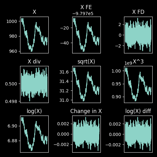
Note – the link between FD, Feature Division, Change, and log: Remember that in general: \( \log(a) – \log(b) = \log(\frac{a}{b}) \). This should help you see how the listed transformations are all actually linked.
Testing your forecasting model
The importance of your error function
When we presented OLS, we first talked about how best to place a line in a scatter of points. We later explained how this decision is essentially made by defining our error. More accurately, the decision is made by how we minimize our defined error. In a traditional Machine Learning course, instead of focusing on defining a linear function and looking at the assumptions needed to make our estimator good, we start with a function that we want to minimize and we see how well it performs.
In fact, in general, ML spends a lot of time thinking about which error function is optimal for which problem. Deciding on your error function to minimize effectively changes your forecasting approach. Even more than that, how you solve that minimization problem can change your forecasting approach. As a result, ML cares a lot about how to solve those minimization problems.
You will often hear talk about the shape of your problem being good, which refers to the geometric shape of the error function to minimize being well-behaved, i.e. being easily differentiable (not having kinks and being smooth), and having easy-to-find optima. This is important because unlike our analytical solution for the OLS estimator, ML wants to be able to minimize arbitrary functions. As such it concerns itself with numerical solutions as opposed to analytical ones.
A formal mathematical exploration of these terms and numerical solutions is out of the scope of this guide, but the intuition is that it’s easier to find a max or a min on a smooth curve than on a curve with lots of sharp twists and turns, and that different approaches deal with sharp twists and turns more or less well.
For the curious, and in no particular order, here are some numerical optimization algorithms to look up:
- Stochastic Gradient Descent
- Adam
- Nesterov Momentum
- Adagrad
- Adadelta
There are a lot of heuristics and methods guiding how to write your own error function, choosing the right optimizer, and optimally training your model. I encourage you to look at the extra resources listed at the end of the guide if you want to learn more about this topic.
On the importance of train-test splits and cross-validation
One of the most useful techniques from Machine Learning is the train-test split. Like many other ML methods, its focus is on improving out-of-sample performance by reducing overfitting. The core idea is to separate your data into two parts. Using your training data, you fit your model the way you usually would. But measuring the performance of your model on your training set could easily lead to over-estimating your goodness of fit by fitting too closely to that specific dataset. Therefore, we measure the validity of the model on a separate, not-before-seen, testing data set. The training data is biased one way or another, and in fact the out-of-sample data is also biased one way or another. The reason why the out-of-sample bias is better is because a priori, not having trained on it, our model is equally likely to perform better or worse on it. That bias is much easier to live with than overfitting bias.
You can also divide your data into more chunks, usually a train, a validate, and a test set (note the terms validate and test are used interchangeably across different textbooks). That way you train your model on your train set, you pick the best (hyper)parameters for that model on your validate set, and you pick the best overall model on the test set. Separating the data between the part we know and the part we don’t know for each decision ensures that we don’t overestimate how much we actually know about unknown future data.
To measure a model’s performance, more data is always better because it gives you more confidence in the measure of the performance. Therefore, losing some of your data to training reduces your certainty on how well your model will perform. Using only a test set means that you sacrifice how confident you are in your test to be more confident about your lack of overfitting bias. So really there are two different types of biases we are juggling: the bias of our measure of fit and the bias of our out-of-sample performance. With less data to test over, our confidence in our performance is lower, but we have more confidence that whatever bias the test set has is symmetric, neither overestimating nor underestimating performance a priori.
Cross-validation aims to solve the problem of the test set being too small to gain good confidence. It works by randomly selecting data points in any order to form a subset of your data. That subset is then split into train and test and your model is fitted and evaluated. This process is repeated many times, sometimes hundreds of times for larger datasets. Each of these subset is called a fold. Then you use the average of your many test measures of fit across all your folds as your overall measure of fit. This method effectively resamples your data to maximally exploit its stochastic nature, as if you were drawing samples from the population many times.
Although cross-validation is very powerful to get a better (i.e. less biased, less over-fitted) measure of fit, you must exercise care when using it. If you measure on the same testing set again and again, in the end the test set becomes part of your training data and is no longer out-of-sample. Therefore, if you resample your data so many times that you train and test over your entire data set hundreds of times, your cross-validation approach will actually result in overfitting.
Of course, everything we just discussed becomes even harder when applying it to time series.
Cross-validation for time series
The time series nature of your data needs to be respected for your model to properly capture the signal you want. As such, the cross-validation step of randomly selecting your data in any order destroys any hope of training a sensible model. There are a variety of ways of still performing cross-validation, but fundamentally they all amount to selecting a block of data instead of selecting data randomly. Then you move that block of data across time. The decisions to make revolve around: how much data goes into each block, how much do you move the block across for the next fold, and how often do you retrain.
Note – A well-specified model: It is not impossible that the features you define for your model specify it so accurately that you can omit the time aspect of your data. In practice, I’ve never seen this to be the case, but I have seen many cases where there wasn’t enough data to work with and so pushing the analysis with this assumption was better than not doing anything.
I explore some time-series cross-validation options below:
- How much data goes into each block
Typically speaking, for any given data set, you would set aside between 60% and 70% of your data for training, and the rest for testing. If you need a validation set, then typically you would use 60% of your data for training, 20% for validating, and the final 20% for testing.
Sometimes there are constraints inherent to your business case: you need to predict your data for the next 24 hours, or you know that the quality of your predictions goes down exponentially the further out you try to predict. In those cases, the more time between train and test, the worse your performance will be. Then, training can be done on a majority of the dataset, while validating and testing are done on very small datasets. Ideally validating should still take about 10% of your data. The small size of your testing set is compensated by having many such folds.
In absolute numbers, having between 500 and 1 000 data points in your training set is good for most OLS applications. If the problem is very complex and has many features (say more than 10 or 15), then you would want at least 10 times that amount of data. Methods like Random Forests tend to perform worse than OLS on very small datasets (e.g. 500 and lower) but perform better on larger ones (e.g. 10 000 and higher). - How to move the block
Let’s offer a concrete example: let’s assume you train your model on your data from index 0 to 100, then validate on index 101 to 120, and then test on 121 to 140.
- Approach 1: move only by the amount that is in your test set. That means that your next fold will train on index 20 to 120, validate on 121 to 140, and test on 141 to 160. You almost never want your test sets to overlap. If they do, you are effectively counting the performance of your model on the same data twice, and so now that piece of data is disproportionately represented in your final goodness of fit.
- Approach 2: move by the entire block, so that you don’t even train on part of the same data at all. This is to avoid issues where an outlier event in that dataset gets fitted many times. Using our above examples, the second fold would train on indeces 141 to 241, then validate on 242 to 261, and test on 262 to 281. Of course, this means we have fewer folds available to measure how well our model is performing.
- Approach 3: move by an amount between the two extremes above. Using the above example, it’s possible for the second fold to reuse half of the training set while still making sure that the new test set is completely new. This can be a good compromise when there isn’t a lot of available data. Using the same example, let’s move by half the training set, knowing that that still covers the testing set and then some. We train on 50 to 150, we validate on 151 to 170, and we test on 171 to 190.
- How often to retrain: Retraining is intricately linked to how you update your train-validate-test split. In the above examples, I implicitly assumed that your retrained for each testing phase. However sometimes this is not computationally feasible, either because the model is too costly to train or because of some data restrictions. Yet we might still want to validate and test in blocks. Testing for model decay becomes very important, and there are ways to test for it. The basic idea behind measuring model decay is to look at the pattern of the model’s performance. If the performance drops off very badly every time three test sets down the line, you know that you will need to retrain your model that often, or else live with worse predictions for a while.
Hypothesis testing
There are plenty of tutorials online that explain how to perform a simple z-test or how statistical significance works. Instead I want to focus on the logic of hypothesis testing, what such a test can tell us, and most importantly what it can’t. Fundamentally, hypothesis testing is a framework for asking questions about our data which must always be in the following form: given the data that I have and what I assume to be true about it, how unlikely are other options?
Precise language for a difficult problem
A hypothesis test starts with your data, a null hypothesis \( H_0 \), and an alternative hypothesis \( H_a \) (sometimes also \( H_1 \)). The first step is to properly define \( H_0 \) and \( H_a \) to fit your problem. Once their definition is set, you assume that \( H_0 \) is true. Then you ask: how likely is it that \( H_a \) is true if \( H_0 \) is true? You can answer this question by calculating a test statistic representing \( H_a \).
Now here’s the key bit: you can never say that \( H_0 \) is true or false; you can never say that \( H_a \) is true or false. It might sound like you can, but really here we are using messy English language to convey very formal mathematical ideas. Many people make this mistake, and the consequences can be dire if you don’t fully understand this distinction. Instead you can say one of two things:
- Either: having seen a result as adverse as our data, with a level of adversity defined by \( H_a \), I can reject the assumption that \( H_0 \) is true. Notice the distinction? We don’t know that \( H_0 \) is true or false. However we know how likely it is to see a result like \( H_a \) if \( H_0 \) is true, so we can reject the null but we cannot say it is untrue.
- Or: to a certain degree, as defined by \( H_a \), and given our data, I cannot reject the null hypothesis that \( H_0 \) is true. Once again, we are not saying that \( H_0 \) is true or false, but simply to what degree the observed data isn’t adverse to the null being true if it is.
Note – Making your own hypothesis tests: most modern statistical packages will let you run all the most common hypotheses tests like an F-test or a t-test, but if you want to learn how to make your own, I highly recommend reading through The Simple and Infinite Joy of Mathematical Statistics.
Note – The Bayesian counterpart to confidence intervals: A Bayesian approach uses distributions as measures of uncertainty instead, and so given that distributional assumption you would get a probability distribution for your outcome of interest in the form of a credible interval.
Precision, in a business context
Let’s consider an example: you run a regression to look at the impact of a new type of bus tyre on the vehicle’s fuel efficiency. You estimate that all else being equal, the buses with the new tyres save on average 5% of the total fuel. You want to test the hypothesis that actually, the true effect of the tyres is 0 or even negative. Then you set \( H_0 \) to be that the true effect is non-positive, and your \( H_a \) is the effect you found.
When you calculate the probability of \( H_a \) being true assuming \( H_0 \) is true, you can build confidence intervals around the value that you found. In the example above, an interval of \( [0.04, 0.06] \) around our estimate would give us strong confidence that our point estimate of 5% is solid, while a confidence interval of \( [-0.07, 0.07] \) might not because it is much wider and it contains negative values. What if the true effect is actually the other way around?
In a sense, the size of the confidence interval is the most interesting aspect of the hypothesis test and is directly tied to the idea of statistical significance. Let’s say that for each percentage point of fuel efficiency, our business will make an extra million dollars. Then a confidence interval of order of magnitude 0.02 as above might not be precise enough, as it implies an error margin of 2 million dollars. But then again, one of order of magnitude 0.14, swinging in the negatives and positives, is even worse.
Often times, the variance of our estimate is a key factor in obtaining our confidence interval, so it’s no surprise that people interpret these intervals similarly. However, a confidence interval isn’t the probability that my estimate is in between two values. To understand what it really is we need to discuss the idea of repeated sampling.
Note – Is my effect 0? Historically, we cared a lot about whether an effect was “real” or not, meaning how sure can I be that the true effect isn’t 0? This question about the point estimate was translated as: does my confidence interval include the value 0? Nowadays we care a lot more about the entire interval resulting from the null and alternative hypothesis.
Repeated sampling
Hypothesis testing comes from the frequentist world and derives fundamentally from the idea of repeated sampling. That is to say, if we were to sample data from the population many times, then our certainty or precision is about how many of these samples would reject or fail to reject the null hypothesis under the assumption it is true. The precision isn’t about the single sample we did get.
So with a classic 95% confidence interval, in repeated samples, we would expect to reject the null 5% of the time. Because 5% isn’t “often”, if it happens in our given sample, we reject the null. But what if we test a million different null hypotheses until we find one we can reject? Then we’re data mining.
Defining different courses of action
So a confidence interval isn’t quite a precision, it’s not quite a distribution, and it doesn’t tell me what is true? So what is it good for?
Consider the following scenario: you try to predict a stock price using an Elastic Net. Filling in your features, you predict that tomorrow’s price will be 2% higher than today’s price. You run an F-test and you get confidence intervals for all your regression coefficients \( \hat{\beta} \).
Let’s assume a very simple set-up: \( price_{t+1} = \beta \times price_{t} + \varepsilon_t \). Then can I just replace \( \beta \) with an interval and get an interval for my next price prediction? In practice, many do this, but mathematically this interval isn’t a distribution, so you have no clue about which part of the confidence interval you should expect to be in. Is the mass of the distribution in the interval near the middle? Near the edges? Without knowing that, a grid search through the interval would be incomplete.
A better use of the interval is to come up with different scenarios: we know \( \beta \) can take values in a given interval, such that if \( \beta \) is below a certain threshold, we want to perform action A, and if it is above, we want to perform action B. Let’s say action A corresponds to \( \beta \) being within a 90% interval around our predicted value, while action B corresponds to being outside of that interval. We know that 90% of the time action A should be correct under the null hypothesis while action B should be correct the rest of the time.
Note that we’re not saying that one value of \( \beta \) is correct, but that in repeated samples we expect the value of \( \beta \) to be in a given interval 90% of the time.
Then, for the next sample, i.e. for tomorrow, we can hedge our bets by assuming there is a 90% chance we will have to perform action A and a 10% chance we will have to perform action B. If we can define these actions on a continuum (say buy some shares of asset A or some shares of asset B), then we can perform 90% of A and 10% of B (or whatever split results in an expected value of 0).
Recent controversies in data mining
In the last 15 or so years, hypothesis testing has become controversial because it makes it easy to perform p-hacking.
The value p in this context is the power of your hypothesis test, in short how adverse \( H_a \) is to \( H_0 \). This value is called the significance of the test, and in many applied fields like economics, your research papers are much more likely to get published if your results are statistically significant. This creates a perverse incentive to achieve statistical significance.
It turns out that by adding or removing just a few strong outliers to/from your data, you can achieve statistical significance at arbitrary levels. This is bad because hypothesis tests form the crux of a lot of estimation.
This issue can’t be fully circumvented, because hypothesis tests react poorly to data mining. The central limit theorem is built into a lot of hypothesis tests when we assume that \( H_0 \) is true, which means that any result obtained this way can be exploited by choosing a deceptive subset of your data.
The details as to how this happens are outside the scope of this guide. For the curious, here is a famous paper that covers a lot of the issues with hypothesis testing: Why Most Published Research Findings Are False, 2022, Ioannidis, PLOS Medicine. For even more details, the following course covers in deep detail the issues with hypothesis testing. For a short summary of the conclusions of that course, see here.
Some examples of algorithms
The table below organizes methods by type:
| Regression | Classification | |
| Supervised | OLS, Lasso, Ridge, Random Forest, Seasonal Decomposition, Generalized Least Squares, Generalized Linear Models, Bayesian Networks, Instrumental Variables Estimation, ANOVA, Kalman filtering | Logit, Probit, LDA, SVM, K-nearest-neighbors |
| Unsupervised | Principle Component Analysis, Markov Autoregression, | K-clsuters, Hidden Markov Models |
References
- On Ridge Regression: https://online.stat.psu.edu/stat508/lesson/5/5.1
- On Lasso 1: https://online.stat.psu.edu/stat508/lesson/5/5.4
- On Lasso 2: https://en.wikipedia.org/wiki/Lasso_(statistics)
- On Elastic Net: https://en.wikipedia.org/wiki/Elastic_net_regularization
- On OLS as a projection: https://medium.com/@vladimirmikulik/why-linear-regression-is-a-projection-407d89fd9e3a
- On defining norms: https://en.wikipedia.org/wiki/Norm_(mathematics)
- On logit: https://en.wikipedia.org/wiki/Logistic_regression
- On GLM: https://en.wikipedia.org/wiki/Generalized_linear_model
- On K-Means: https://en.wikipedia.org/wiki/K-means_clustering
- On KNN: https://en.wikipedia.org/wiki/K-nearest_neighbors_algorithm
- On SVM: https://en.wikipedia.org/wiki/Support_vector_machine
- On Decision Trees: https://en.wikipedia.org/wiki/Decision_tree
- On unit roots 1: https://stats.stackexchange.com/questions/608174/why-exactly-is-a-unit-root-a-problem
- On Unit roots 2: https://en.wikipedia.org/wiki/Unit_root
- On the characteristic equation: https://en.wikipedia.org/wiki/Characteristic_equation_(calculus)
- On stationarity: https://en.wikipedia.org/wiki/Stationary_process
- On autocorrelation: https://en.wikipedia.org/wiki/Autocorrelation
- On the ADF test: https://en.wikipedia.org/wiki/Augmented_Dickey%E2%80%93Fuller_test
- On the KPSS test: https://en.wikipedia.org/wiki/KPSS_test
- On Fixed Effects (FE): https://en.wikipedia.org/wiki/Fixed_effects_model
- On First Difference (FD): https://en.wikipedia.org/wiki/First-difference_estimator
- On the Adam optimizer: https://machinelearningmastery.com/adam-optimization-algorithm-for-deep-learning/
- On debates around hypothesis testing 1: https://stats.stackexchange.com/questions/10510/references-containing-arguments-against-null-hypothesis-significance-testing
- On debates around hypothesis testing 2: https://journals.plos.org/plosmedicine/article/info:doi/10.1371/journal.pmed.0020124
Leave a Reply