Stochastic Linear Programs

June 4, 2026

Introduction #

I’m fairly new to the topic of linear optimisation (or linear programming as the cool kids say), and coming from statistics my immediate thought was: what happens if I throw a random variable in there? There is such a thing as stochastic programming, but if my wikipedia reading skills don´t betray me, it amounts to maximising a function which contains an expected value operator, which isn’t quite what I’m interested in.

Instead, I want to transfer the uncertainty I have about my inputs into my outputs more directly. In a (kind of) Bayesian sense, if I have a distribution (maybe an empirical distribution obtained via resampling, maybe a distribution obtained via MCMC methods) for my input data, can I get an output distribution for the value of my objective function or for the value of the variables?

In this post, I’ll generate some data from some known distributions, feed it through an optimisation program, and see what comes out!

Speedrun #

Here’s the github repo with the code.

Linear programs (LPs) have some nice stability properties. Their N equations define a polygon in N-d-space, and their solutions lie on the edges of that polygon. However, this stability doesn’t extend to the values of the variables - unsurprisingly - or to the shape of the objective value’s distribution - even in seemingly trivial cases. Not only that, we’ll see that even for a distribution as “simple” as a normal, we need quite a few data points before we can make any statements.

Some vocabulary #

Just so we’re all on the same page, I will use the following conventions:

Program: in this blog post ‘program’ will mean ‘optimisation program’ (as opposed to computer program)
Modelling language: the library that I write the model in
Parameters / data: to refer to everything the program takes as given
Variables: to refer to the decision variables the program has control over
Constraints: to refer to the program’s constraints
Objective: to refer to the program’s objective function to maximize or minimize

Choice of modelling language and optimiser #

For several years I’ve been working with HiGHS, but never got to try its dedicated python interface, highspy, so that’s what I chose. HiGHS is great because it’s the first open-source solver to even approximate the performance of the closed-source stuff like gurobi. I’ve met the HiGHS team several times and they’re really great people, both very smart and dedicated to creating the highest quality open source solver they can. In the past, at work I used pyomo extensively. It’s very powerful because it’s backend agnostic, meaning you can plug any solver into it, but it now feels somewhat dated and is having to deal with its own tech debt. My favorite part about it is how it follows the python convention that everything is an object so you can do all sorts of python wizardry with it. Other contenders are linopy, which is much faster at building models, and cvxpy, which is used for convex programming (but now uses HiGHS, and especially its recent HiPO solver).

Model set-up #

We’ll look at just two simple models and see if we can reason analytically about them.

Simple sum #

The first model just takes two variables and maximizes their weighted sum based on two parameters. The only constraints are on the bounds of the variables. As we’ll see, even such a simple model has some surprising behaviors.

\begin{alignat*}{0} & \max_{x_0, x_1} x_0 \times a + x_1 \times b \\ & \text{s.t.} \\ & x_0, x_1 \in [0,1] \end{alignat*}

Here’s how that looks in code:

def sum_model(a: float, b: float):
    """
    Always sets x0 and x1 to their max value
    """
    h = highspy.Highs()
    x0 = h.addVariable(lb = 0, ub = 1)
    x1 = h.addVariable(lb = 0, ub = 1)

    h.maximize(a * x0 + b * x1)

    h.run()

    solution = h.getSolution()
    num_vars = len(solution.col_value)

    col_value = list(solution.col_value)
    value = [col_value[icol]
             for icol in range(num_vars)]

    return value, h.getObjectiveValue()

We expect this to always set the variables to their maximum values.

Constrained sum #

The second model adds just a simple constraint that the variables:

\begin{alignat*}{0} & \max_{x_0, x_1} x_0 \times a + x_1 \times b \\ & \text{s.t.} \\ & x_0, x_1 \in [0,1] \\ & x_0 + x_1 - 1 == 0 \end{alignat*}

In code, we add just one line to the previous model:

h.addConstr(1 == x0 + x1)

This time, we expect only the variable with the highest weight to be set to 1, while the other variable is set to 0.

Monte Carlo #

Now that we have our models, we generate many samples of the weights $a$ and $b$ :

def loop_sum_model(loc: float, scale: float):
    rng = np.random.default_rng(0)
    params = rng.normal(loc=loc, scale=scale, size=(1000,2))
    xs = []
    objectives = []
    for param in params:
        x, obj = sum_model(param[0], param[1])
        xs.append(x)
        objectives.append(obj)

    theoretical = np.sum(params, axis = 1)
    fig, ax = plt.subplots(1, tight_layout=True, figsize=(10,10))
    ax.hist(objectives, bins=50, alpha=0.7, color="blue")
    ax.hist(theoretical, bins=50, alpha=0.7, color="green")
    fig.savefig(f"sum_model_{loc}_{scale}.png")
    plt.close()

(The loop for the constrained model is almost identical, except the theoretical variable.)

First results #

What do we expect will happen? Both models have the same objective function, which as written looks like we’re summing two normal distributions. So we should expect the objective function to be a sum of normals. Here’s what it looks like running loop_sum_model(0.0, 1.0):

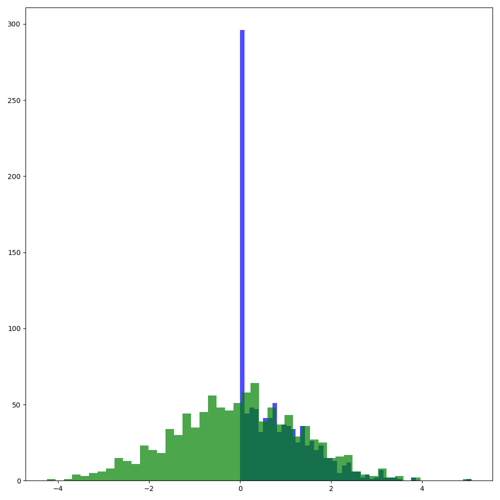
loop_sum_model(0.0, 1.0) — Sum model with peak at 0

The theoretical and the actual distribution disagree! What’s happening? The constraint on the bounds of our variables, along with the maximization objective, is playing tricks on us. If the parameters we sample are negative, which happens about half the time with a normal distribution centered on $0$ , then to maximize the objective, it is better to set both variables to $0$ .

Running instead loop_sum_model(100.0, 1.0):

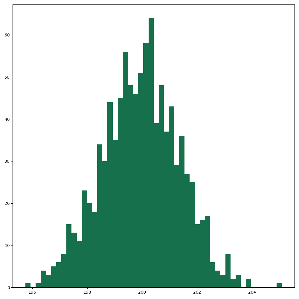
Which fits our intuition because there is no pesky sign change. Although unlikely with this combination of mean and variance, consider in general that 6 standard deviations (e.g. 3 up or down) happens once in every 1000 draws. Depending on your use case, you might not be able to ignore the peak at 0, or change the mean arbitrarily.

The harder model looks even weirder #

The constrained model seems like it should just be a sum of normals, and so a normal again. Let’s run loop_constrained_sum_model(100.0, 1.0, 1000):

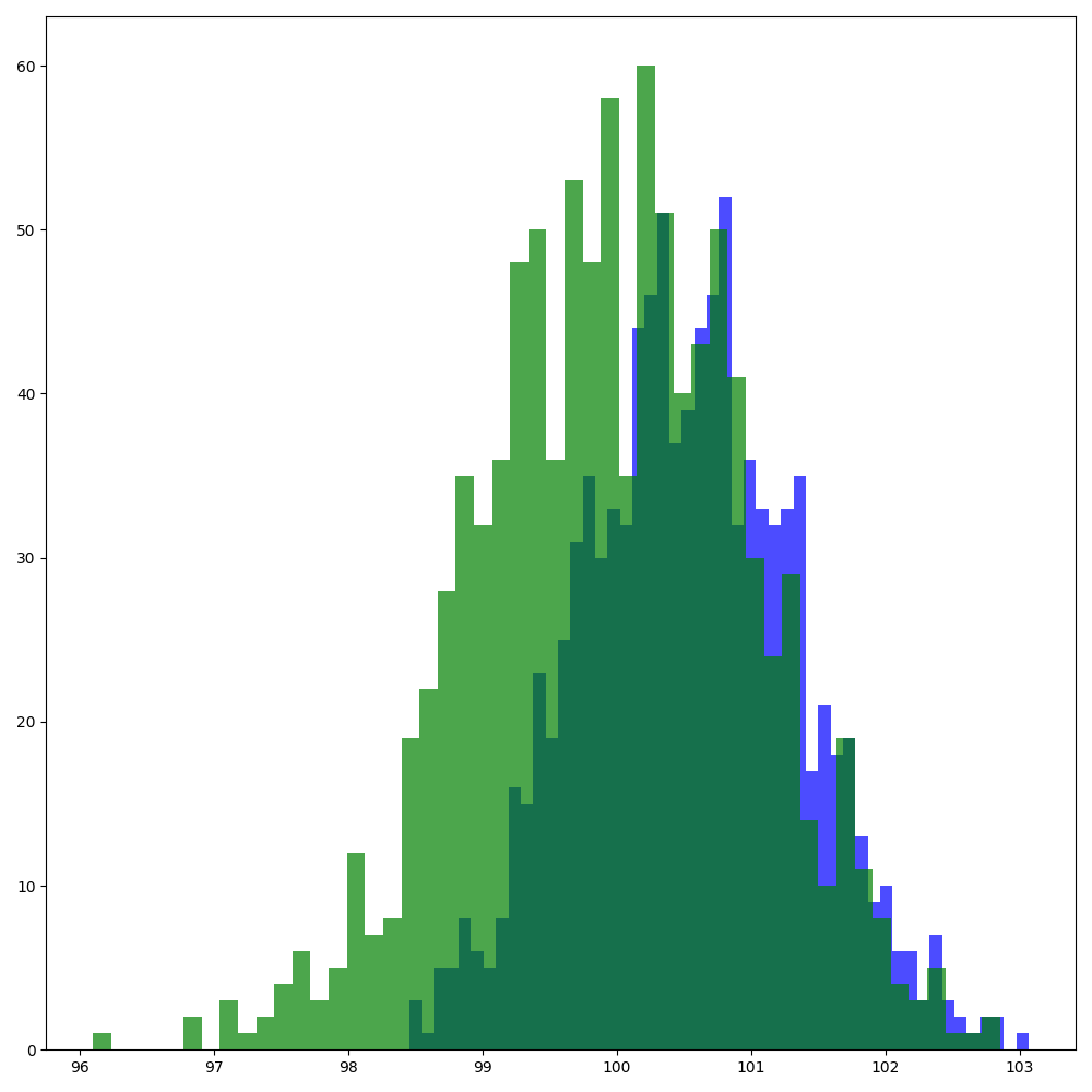
The distribution looks okay and has no weird peaks, but it’s shifted. What gives?

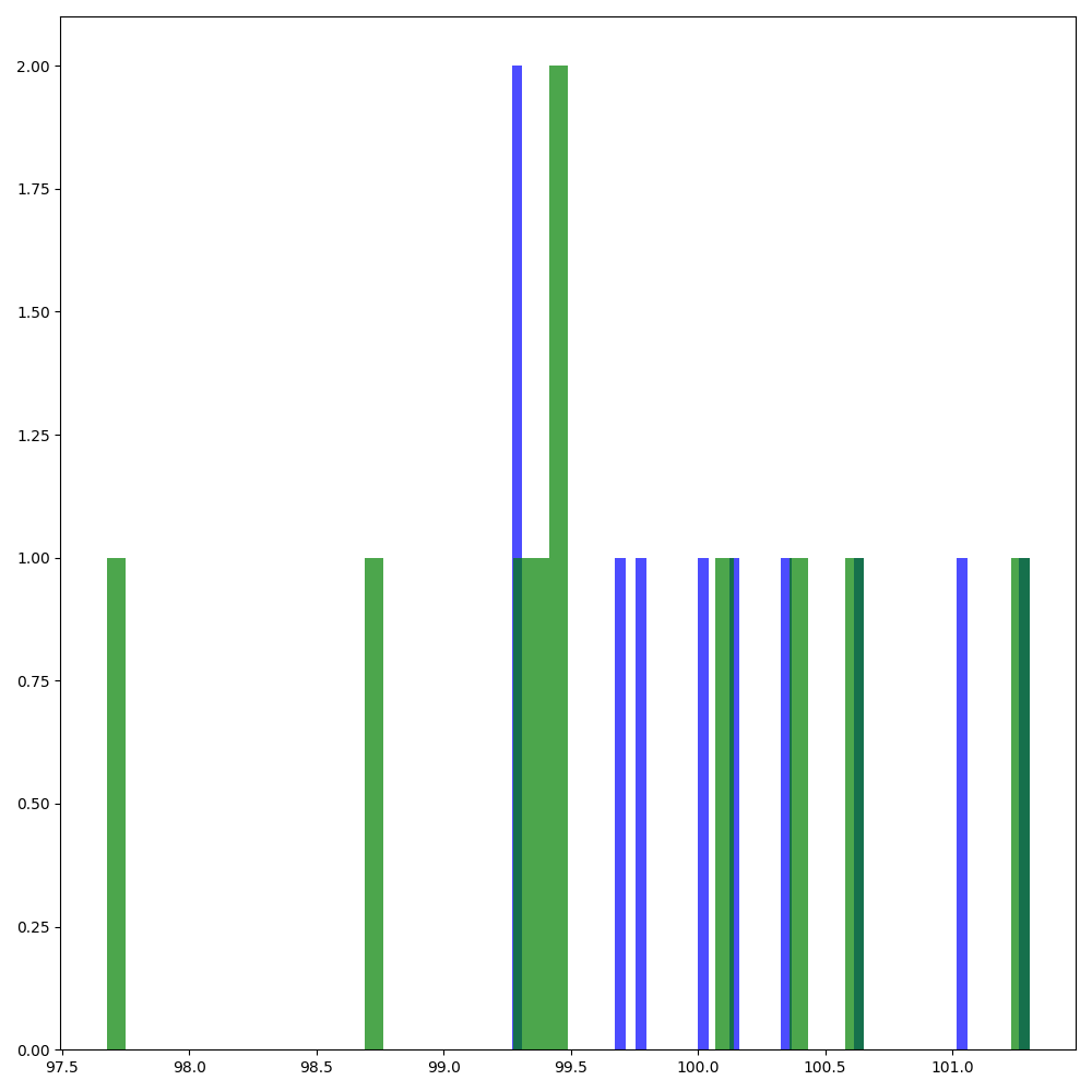
The optimizer only ever sets to 1 the variable with the highest weight, so the sample distribution we’re getting is based on $Pr(a) < Pr(b)$ which sets us to about a mean of $100.5$ . The tricky bit here is that this is only obvious after running many iterations. 1000 is not a small number of steps for a non-trivial LP. Look at 10:

constrained_sum_model(100.0, 1.0, 10) — Constrained sum model, 10 samples

And at 100:

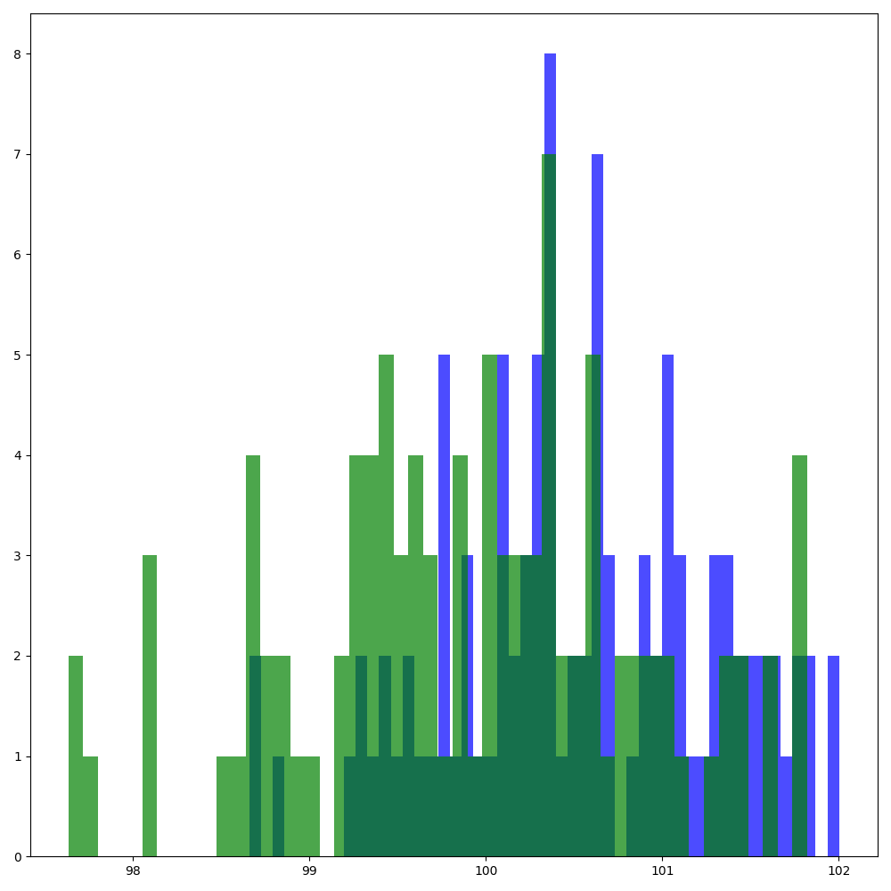
constrained_sum_model(100.0, 1.0, 100) — Constrained sum model, 100 samples

These look like they could be from the same distribution, and a simple graphical test isn’t enough.

Beyond the plots #

Using a Kolmogorov-Smirnov test test, let’s compare. If you’re not sure what this test does or how hypothesis testing works, see wikipedia or my forecasting guide.

We just add the line:

test = scipy.stats.kstest(objectives, theoretical)

Then running for all the different variations of the two models seen so far, we get:

Sum - loc: 100.0, scale: 1.0
KstestResult(statistic=np.float64(0.0), pvalue=np.float64(1.0), statistic_location=np.float64(195.75138424208478), statistic_sign=np.int8(1))

Sum - loc: 0.0, scale: 1.0
KstestResult(statistic=np.float64(0.502), pvalue=np.float64(6.103857836584651e-115), statistic_location=np.float64(-0.006337541033565708), statistic_sign=np.int8(-1))

Constrained - loc: 100.0, scale: 1.0, num_elems: 10
KstestResult(statistic=np.float64(0.4), pvalue=np.float64(0.41752365281777043), statistic_location=np.float64(99.46433062683889), statistic_sign=np.int8(-1))

Constrained - loc: 100.0, scale: 1.0, num_elems: 100
KstestResult(statistic=np.float64(0.29), pvalue=np.float64(0.0004117410017938115), statistic_location=np.float64(100.07559361074289), statistic_sign=np.int8(-1))

Constrained - loc: 100.0, scale: 1.0, num_elems: 1000
KstestResult(statistic=np.float64(0.255), pvalue=np.float64(5.77199391392635e-29), statistic_location=np.float64(99.97384321347702), statistic_sign=np.int8(-1))

In a KS test, the null hypothesis is that the distributions are the same.

For the first test, we know that theoretically the two distributions are identical, and in practice the plots perfectly line up, so it’s no surprise that we cannot reject the null.

The second test, the one with the spike, has a really small p-value, and so we can reject the null.

The third, fourth, and fifth tests, show us that as the sample size increases, the p-value decreases. For 10 elements, we can’t reject the null, but starting at 100 we can be pretty certain, despite the plot being a coin toss. And of course as seen in the plot, after 1000 draws the distributions look very different.

Conclusion #

Although LPs have some nice stability properties, reasoning about the distributional properties of their objectives is difficult even in simple cases. Moreover, the values of the variables can be maximally different despite the objectives being close to each other, and this for minimally different values of the parameters. Finally, they require a fairly large sample size and hypothesis tests before we can be sure.